Analyzing UK election tweets in R using RSQLite and quanteda
This is a small project that I completed as a part of one of my masters degree courses. It uses data from the 2017 UK General Election campaign. The dataset contains tweets posted by candidates and political parties, and replied to those tweets.
First, load the necessary libraries.
library(DBI)
library(RSQLite)
library(quanteda)
library(quanteda.textplots)
Connect to the database.
db <- dbConnect(RSQLite::SQLite(), "uk_election_tweets_small.sqlite")The database contains two tables, “users” and “tweets”. Let’s access them and get an idea about the number of observations in each.
#Number of rows in the tweets table
dbGetQuery(db, 'SELECT COUNT(*) FROM tweets')

#Output: 22130

#Number of rows in the users table
dbGetQuery(db, 'SELECT COUNT(*) FROM users')

#Output: 5572
In our datasets we have some indicator columns: in_reply_to_screen_name_in in the “tweets” table indicates whether a tweet is a reply to a politician or a political party; screen_name_in in the “users” table is equal to 1 if an account belongs to a politician or a party, and 0 otherwise. Let us also use them to get some insights from our data.
#How many tweets are replies to politicians/parties?
dbGetQuery(db, 'SELECT COUNT(*)
           FROM tweets
           WHERE in_reply_to_screen_name_in = 1')

#Output: 1829

#How many accounts are from politicians/parties?
dbGetQuery(db, 'SELECT COUNT(*)
           FROM users
           WHERE screen_name_in = 1')

#Output: 1055

#How many accounts are from other users?
dbGetQuery(db, 'SELECT COUNT(*)
           FROM users
           WHERE screen_name_in = 0')

#Output: 4517
Let us also analyze the accounts in our database from the perspective of popularity and tweet count.
#Which screen_name has posted the highest count of tweets?
dbGetQuery(db,'SELECT u.screen_name, COUNT(*) as count
           FROM tweets t
           LEFT JOIN users u
           ON u.user_id_str = t.user_id_str
           GROUP BY u.screen_name
           ORDER BY count DESC
           LIMIT 1')

#Output: DrTeckKhong

#Who has the highest number of followers?
dbGetQuery(db, 'SELECT screen_name, MAX(followers_count)
           FROM users')

#Output: RufusHound

#Among politicians, who has the highest number of followers?
dbGetQuery(db, 'SELECT screen_name, MAX(followers_count)
           FROM users
           WHERE screen_name_in = 1')

#Output: jeremycorbyn
It is also interesting to find out what account was tagged the most in our tweets.
#Get only tweets containing tags of users using a query
usertag_tweets <- dbGetQuery(db, "SELECT text
           FROM tweets
           WHERE text LIKE '@%'")

#Document-feature matrix
users_dfm <- tokens(usertag_tweets$text, remove_punct = TRUE) %>%
    dfm()

#Extract user tags and get the most common ones
tag_dfm <- dfm_select(tweets_dfm, pattern = "@*")
top_usertags <- names(topfeatures(tag_dfm, 50))

#The user that was tagged the most
top_usertags[1]

#Output: @midsussex_times
Let’s also get an idea about the time frame of the dataset.
#Earliest time stamp
dbGetQuery(db, 'SELECT text, MIN(created_at)
           FROM tweets')

#Output: Fri Jun 02 00:00:09 +0000 2017

#Latest time stamp
dbGetQuery(db, 'SELECT text, MAX(created_at)
           FROM tweets')

#Output: Wed May 31 21:00:00 +0000 2017
Next we can start analyzing the hashtags in the dataset. Let’s look at the tweets that contain the word “brexit”.
#How many tweets contained the word brexit?
dbGetQuery(db, "SELECT COUNT(*)
FROM tweets
WHERE text LIKE '%brexit%'")
#Output: 1058
#What proportion of tweets by only politicians contained the word brexit? (in %)
dbGetQuery(db, "SELECT CAST(100/(COUNT(*) / (SELECT COUNT(*) FROM tweets t
LEFT JOIN users u
ON u.user_id_str = t.user_id_str
WHERE screen_name_in = 1 AND text like '%brexit%')) AS FLOAT)
FROM tweets t
LEFT JOIN users u
ON u.user_id_str = t.user_id_str
WHERE screen_name_in = 1")
#Output: 4%
#What proportion of tweets by other users contained the word brexit? (in %)
dbGetQuery(db, "SELECT CAST(100/(COUNT(*) / (SELECT COUNT(*) FROM tweets t
LEFT JOIN users u
ON u.user_id_str = t.user_id_str
WHERE screen_name_in = 0 AND text like '%brexit%')) AS FLOAT)
FROM tweets t
LEFT JOIN users u
ON u.user_id_str = t.user_id_str
WHERE screen_name_in = 0")
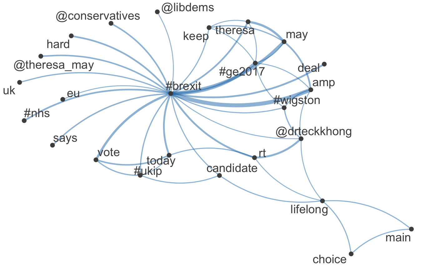
#Output: 5%Further on, our analysis is going to go deeper into hashtags, their relationship between each other and other words. In the next chunk of code I create a function that makes use of the quanteda.textplots package by returning a visualization for the word network of a given hashtag.
Then I am going to select some hashtags that form networks that appears to be interesting or informative and provide illustrations for these networks.
hashtag_network <- function(x){
  #Takes a hashtag, retrieves tweets containing this hashtag, and
  #returns a visualization of the network of this hashtag.
  query <- paste0("SELECT text FROM tweets WHERE text LIKE '%#", x, "%'")
  hashtag_tweets <- dbGetQuery(db, query)

  set.seed(42)
  toks <- hashtag_tweets$text %>%
      tokens(remove_punct = TRUE) %>%
      tokens_tolower() %>%
      tokens_remove(pattern = stopwords("english"), padding = FALSE)
  fcmat <- fcm(toks, context = "window", tri = FALSE)
  feat <- names(topfeatures(fcmat, 30))
  fcm_select(fcmat, pattern = feat) %>%
      textplot_network(min_freq = 0.5)

  fcm_select(fcmat, pattern = feat) %>%
      textplot_network(min_freq = 0.8)
}
Let’s see the visualizations for the selected tweets.
hashtag_network('brexit')
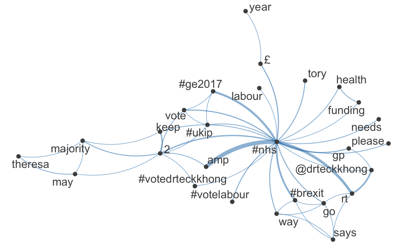
hashtag_network('nhs')
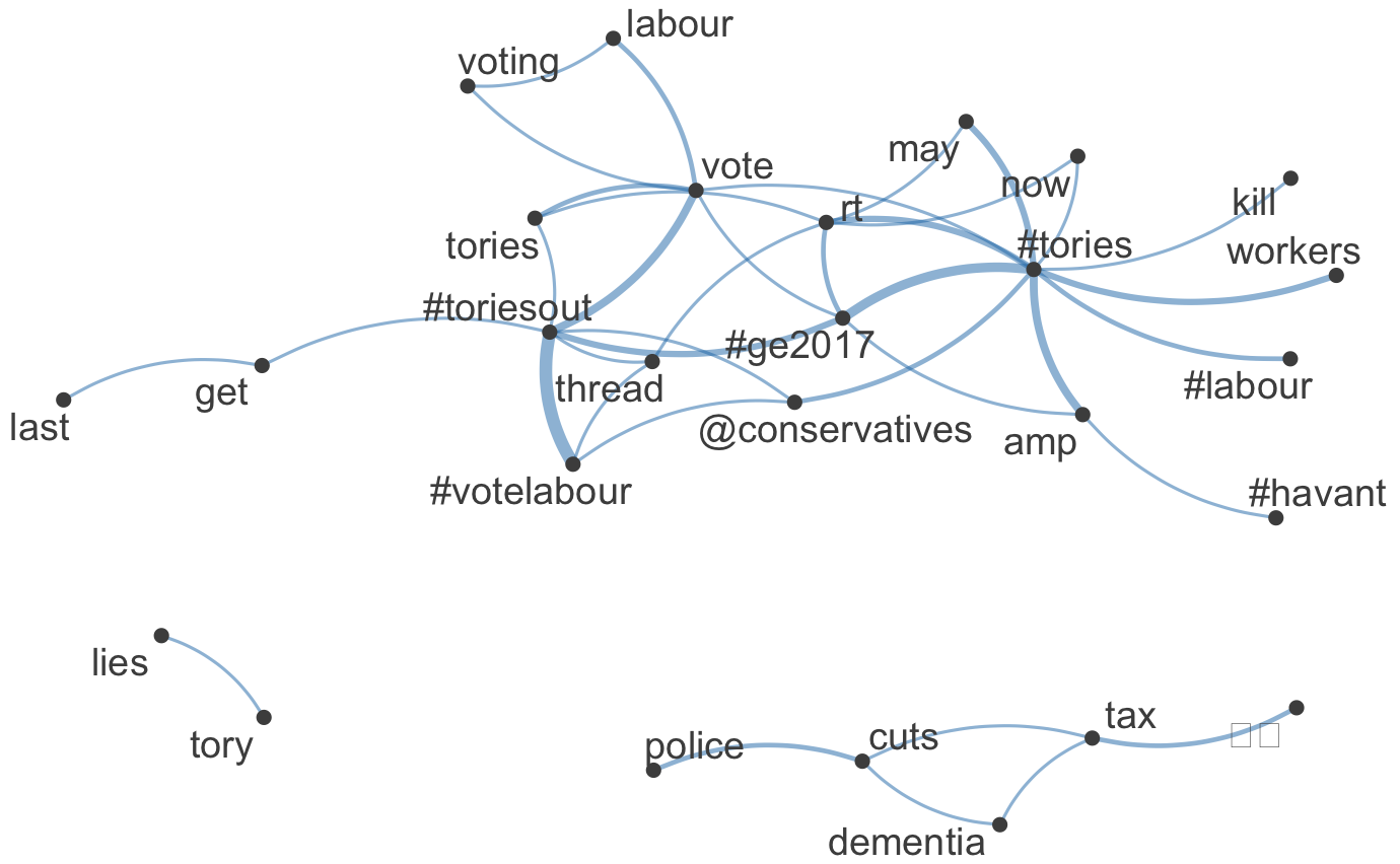
hashtag_network('tories')Network for hashtag "brexit"
Network for hashtag "nhs"
Network for hashtag "tories"
Finally, we need to disconnect from the database.
dbDisconnect(db)