Analysis of song lyrics in popular music using quantitative text analysis techniques
This is a project that I did as my final assignment for the Quantitative Text Analysis graduate course. My primary source of data was the full history of Billboard Hot 100 published weekly, which I retrieved from Kaggle. I then downloaded the lyrics for the songs from the chart using the API of Genius, and gathered some additional information, such as genre and country where the track was released using the API of Discogs.com. Using the quanteda package, I transformed the data into a corpus, treating the lyrics of each song as a separate document, and created a DFM and a tokens object for the respective functions that only accept data in this format. To analyse the lyrics, I implemented topic modelling and keyness analysis. Below I present the code for each step of my project.
Note: racial slurs in plots were blurred out.
First, load the necessary packages.
library(tidyverse)
library(geniusr)
library(stringr)
library(httr)
library(lubridate)
library(quanteda)
library(quanteda.textstats)
library(quanteda.textplots)
library(stm)
library(ggplot2)
Gathering the lyrics using the Genius API (paths and access information for APIs are not shown for privacy reasons):
#import data
tracks <- read_csv("/.../billboard-hot-100-tracks.csv",
                   show_col_types = FALSE)

#set access information for the API
Sys.setenv(GENIUS_API_TOKEN = "TOKEN")

#create empty lists to store information
lyrics_documents <- c()
date_list <- c()
names_list <- c()

for(i in 1:nrow(tracks)){
  #get information for a track
  song <- tracks[i,]
  song_date <- song$date

  print(i)
  try({
    #retrieve a tibble with lyrics for the song
    lyrics_tibble <- get_lyrics_search(song$artist, song$song)

    #concatenate all lines into one string
    doc <- str_c(lyrics_tibble$line, collapse = " ")

    #get the full name of the song to use as the name of a future document
    docname <- str_c(c(song$artist, song$song), collapse = " - ")
    names(doc) <- docname

    lyrics_documents[i] <- doc
    date_list[i] <- song_date
    names_list[i] <- docname
  }
  )
}

#create a dataframe out of the information we retrieved
corpus_df <- data.frame(lyrics = lyrics_documents,
                        date = date_list,
                        names = names_list)

#drop NA values
corpus_df <- drop_na(corpus_df)

#convert date into a proper format
corpus_df$date <- as.Date(corpus_df$date, origin = lubridate::origin)
Downloading data from the Discogs.com database:
#get login information for the API
discogs_key <- 'CONSUMER_KEY'
discogs_secret <- 'CONSUMER_SECRET'

#create empty columns for country and genre to fill them later
corpus_df$genre <- 0
corpus_df$country <- 0

for (i in 1:nrow(corpus_df)){
  try({
      song <- corpus_df$names[i]
      song <- str_remove_all(song, "-")
      song <- str_split(song, " ")
      song <- song[[1]]
      song <- song[song != ""]

      query <- str_c(song, collapse = "%20")

      #create a search query for the API
      search_url <- sprintf("https://api.discogs.com/database/search?q=%s&key=%s&secret=%s", query, discogs_key, discogs_secret)

      #submit the query
      search_r <- GET(search_url)

      search_c <- content(search_r, "parsed")

      #retrieve the country of origin
      s_country <- search_c$results[[1]]$country

      #retrieve the genre
      s_genre <- search_c$results[[1]]$genre[[1]]

      corpus_df$country[i] <- s_country
      corpus_df$genre[i] <- s_genre

      #make a pause to limit the number of requests per minute
      Sys.sleep(1)
  })
}

#store the newly created dataframe as a CSV
write.csv(corpus_df, file='.../df_genre_country.csv')
The original dataset contains charts published from 1959 until 2021, however due to time and API requests limits the dataset I used for this project only contains data from 1995-2021. Overall, it has 60400 observations. The chunk of code below removes rows with missing information and columns that are not going to be used and creates objects that we will use further (corpus, tokens object, and DFM).
corpus_df <- read_csv('/.../df_genre_country.csv',
                      show_col_types = FALSE)

#remove rows where country and genre were not retrieved
corpus_df <- corpus_df %>%
  filter(genre != 0) %>%
  select(-1) #remove the first columns with indices

#create a corpus object out of our dataset
billboard_corp <- corpus(corpus_df, text_field = "lyrics")

#set the names of songs as names of documents
docnames(billboard_corp) <- corpus_df$names

#create a tokens object
toks <- tokens(billboard_corp,
               remove_punct = TRUE,
               remove_numbers = TRUE,
               remove_url = TRUE,
               remove_symbols = TRUE,
               remove_separators = TRUE) %>%
  tokens_remove(stopwords("en"))

#create a DFM object as well
b_dfm <- toks %>%
  dfm(tolower = TRUE)
Topic Modelling
Now we proceed to topic modelling. To be specific, I will be implementing structural topic models for K from 2 to 10, where K is the number of topics. For each of those metrics of semantic coherence, exclusivity, and others will be calculated, based on which I will select an optimal value of K and use the corresponding model for further analysis.
#convert into an input for a structural topic model
stm_input <- convert(b_dfm, to = "stm")

#perform a search over K values
k_search_output <- searchK(stm_input$documents, stm_input$vocab,
                           K = c(2, 3, 4, 5, 6, 7, 8, 9, 10),
                           data = stm_input$meta,
                           verbose = FALSE, heldout.seed = 42)

plot(k_search_output)
print(k_search_output)
Results of K search
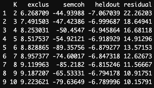
To choose an optimal value of K, a balance needs to be reached between semantic coherence and exclusivity: both need to be maximized, however as K increases, the two metrics change in opposite directions. As we may see, the highest semantic coherence is achieved for K = 2, while highest exclusivity - for K = 10. As for the optimal K, I am inclined to choose between K = 4 and K = 5. Semantic coherence scores of - 50.4547 and -54.92121 are slightly worse than for K = 2, however they are significantly better than for higher values of K. Meanwhile, exclusivity scores of 8.253031 and 8.517537 are a noticeable improvement over the ones for lower values of K. To make the final choice, let us fit models for these values and see for which one the topics make more sense.
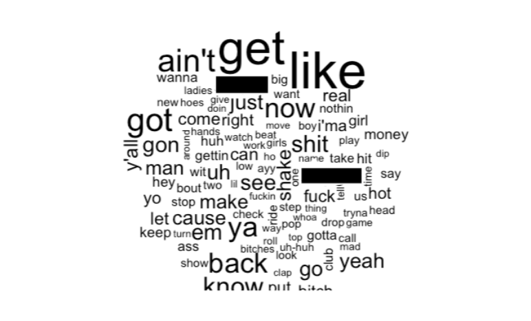
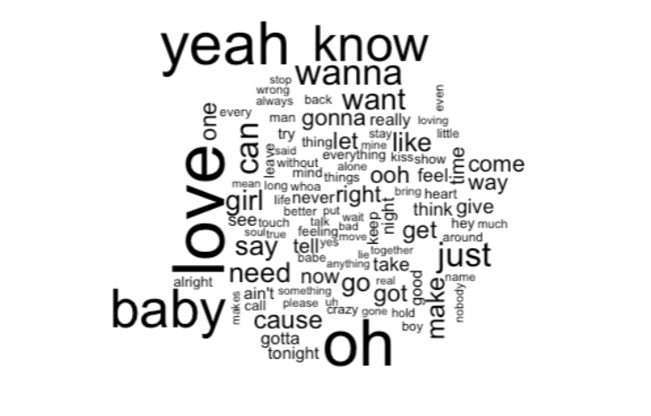
Wordcloud for Topic 1
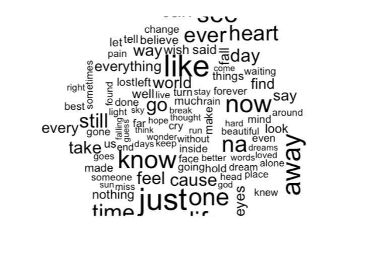
Wordcloud for Topic 2
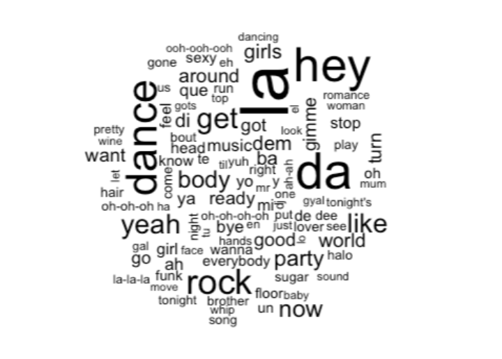
Wordcloud for Topic 3
Wordcloud for Topic 4
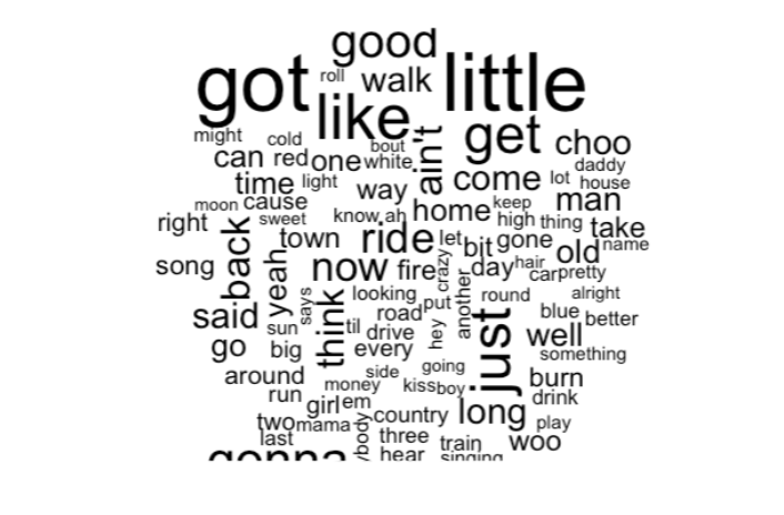
Wordcloud for Topic 5
There is a lot of overlap in topics in both models, however it seems that the identified topics in the model with K = 5 make slightly more sense, so I decided to stick with it. I believe the topics could be characterized as follows:
- slang, curses and slurs (most likely rap/hip-hop lyrics)
- “romantic non-light-hearted”/emotional lyrics
- dancing-related lyrics
- “romantic light-hearted” lyrics
- rather difficult to identify a common theme, however the presence of the words like “ride”, “town”, “car”, etc. indicates that this topic probably relates to country music lyrics or has something to do with travelling
It appears that topics 1, 3, and 4 feature more simplistic language than topics 2 and 5, however more complex analysis is needed to confirm this. Overall, it seems that some of the topics were formed based on typical lyrics in different music genres rather than actual topics in the common sense of the word.
Now we are going to look at the topic distribution across genres and countries.
lyrics_topics <- findThoughts(topic_model_2,
texts = corpus_df$lyrics,
n = 1000)$index
#initialize the data frame
topics_df <- corpus_df[unlist(lyrics_topics[1]),]
topics_df$topic <- 1
#select the most likely songs for each topic and bind them into one dataframe
for (i in 2:length(lyrics_topics)){
df <- corpus_df[unlist(lyrics_topics[i]),]
df$topic <- i
topics_df <- rbind(topics_df, df)
}
#bar chart showing the relationship between topic and genre
plot_genre <- ggplot(topics_df,
aes(x = topic,
fill = genre)) +
geom_bar(position = "stack") +
ggtitle("Share of music genres in each topic")
#bar chart showing the relationship between topic and country
plot_country <- ggplot(topics_df,
aes(x = topic,
fill = country)) +
geom_bar(position = "stack") +
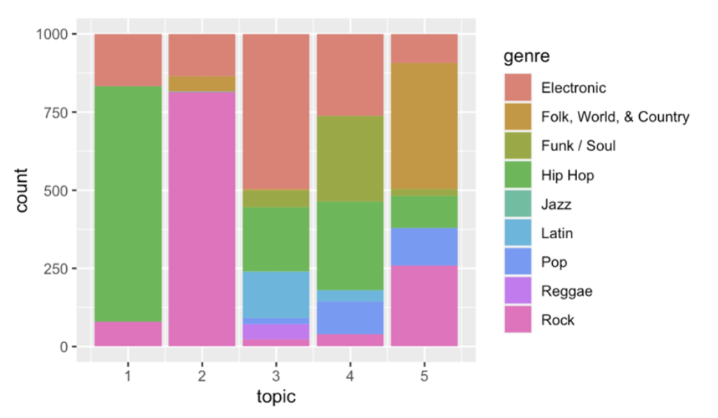
ggtitle("Share of countries in each topic")Share of music genres in each topic
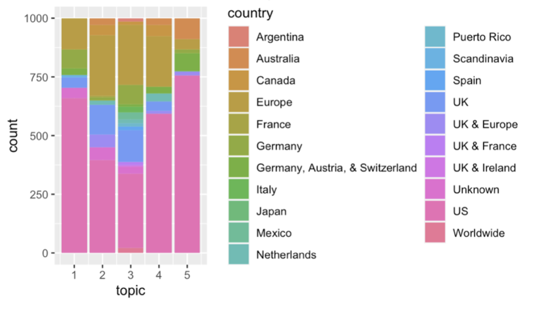
Share of countries in each topic
Let us analyze the plots shown above.
As for the genre plot, we can clearly see that the most common genre for Topic 1 is hip-hop. I have briefly noted above that most likely the words encountered in the wordcloud for this topic relate to this genre of music, which turned out to be correct. Another important thing to note that in Topic 1 hip-hop occupies a noticeably larger share than in others. Hip-hop also occupied substantial shares in Topic 3 and 4 (dance-related lyrics and romantic light-hearted lyrics). Meanwhile, Topic 2 is predominantly rock music, which has a small share in most topics. It also has a substantial, but a much smaller share in Topic 5 (ambiguous, possibly travel-related lyrics).
The other three topics do not have a highly dominant music genre as in the previous two. However, in Topic 3 the most common one is electronic, in Topic 4 it is funk/soul and hip-hop (electronic has a substantial share too), and in Topic 5 it is folk/world/country (with rock having a relatively big share too). Overall, the findings above make sense and confirm some of the guesses made above. To elaborate, we would anticipate that electronic music has dance-related lyrics (Topic 3), funk and hip-hop may have “light-hearted” romantic lyrics (Topic 4), and as was hypothesized, Topic 5 mostly relates to folk/country music. Unfortunately, the plot depicting the country distribution for topics is not as insightful. In most of the topics the biggest share is occupied by the US, which is not surprising since the chart originates from this country. However, probably the interesting thing to note here is that the US occupies the largest shares in Topics 1 and 5, meaning that either hip-hop and country mostly originate from the US, or that people in the US prefer listening to music originating from their own country in these genres. Perhaps, the first is more likely to be the case for country, and how hip-hop it is either the second or a mix of both. Meanwhile, the US occupies the smallest share in Topic 3 which is mostly electronic music; perhaps, this is explained by the fact that a lot of popular electronic music originates from Europe.
Let us take this analysis further and study the genre distribution in each topic across the years.
#extract year from date for simplicity
topics_df$year <- as.factor(format(as.Date(topics_df$date, format="%Y/%m/%d"),"%Y"))
#initialize a column for topic count in each year
topics_df$topic_count <- 1
plot_year_1 <- ggplot(topics_df[topics_df$year %in% levels(unique(topics_df$year))[1:11],]) +
geom_bar(aes(x = topic,
y = topic_count,
fill = genre),
position = "stack",
stat = "identity") +
facet_grid(~ year) +
theme(legend.key.size = unit(0.5, 'cm'),
legend.key.height = unit(0.5, 'cm'),
legend.key.width = unit(0.5, 'cm'),
legend.title = element_text(size=7),
legend.text = element_text(size=5)) +
ylim(0, 200) +
ggtitle("Topic occurrence in 1995-2005, grouped by genre")
plot_year_2 <- ggplot(topics_df[topics_df$year %in% levels(unique(topics_df$year))[12:length(unique(topics_df$year))],]) +
geom_bar(aes(x = topic,
y = topic_count,
fill = genre),
position = "stack",
stat = "identity") +
facet_grid(~ year) +
theme(legend.key.size = unit(0.5, 'cm'),
legend.key.height = unit(0.5, 'cm'),
legend.key.width = unit(0.5, 'cm'),
legend.title = element_text(size=7),
legend.text = element_text(size=5)) +
ylim(0, 200) +
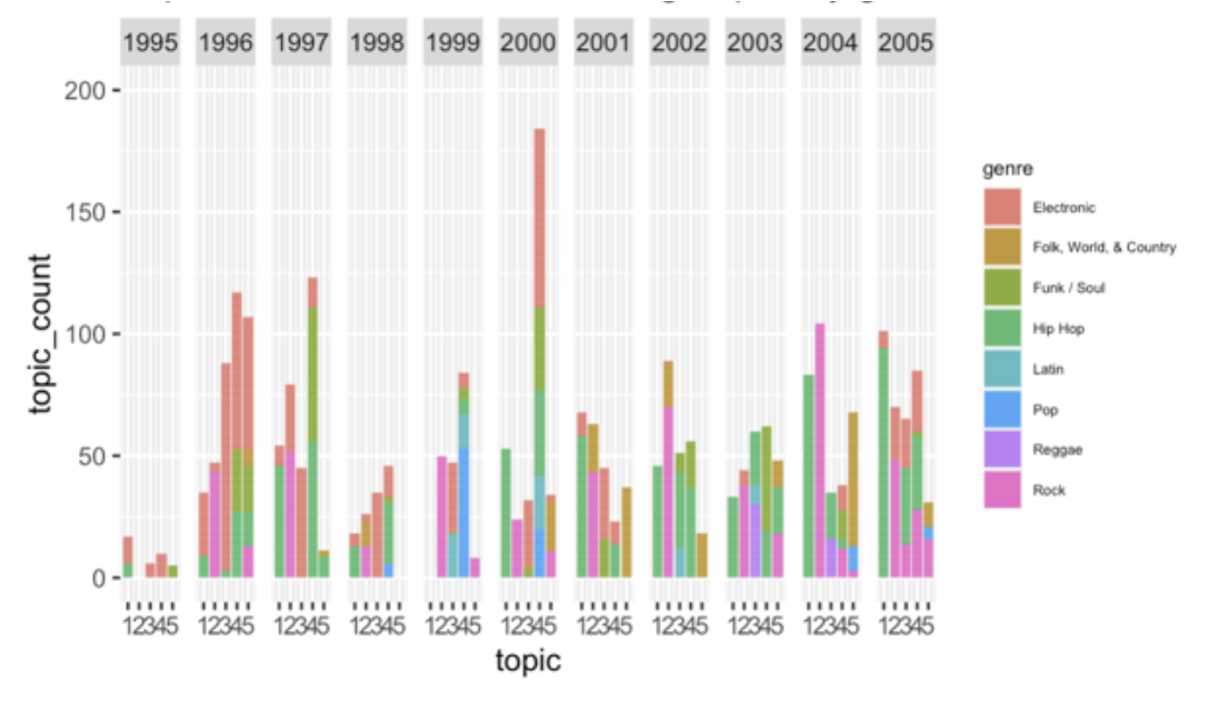
ggtitle("Topic occurrence in 2006-2021, grouped by genre")Topic occurrence in 1995-2005, grouped by genre
Topic occurrence in 2006-2021, grouped by genre
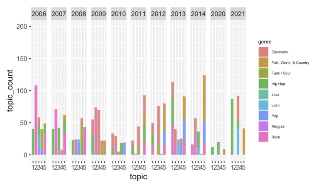
Above I show topic count for each year, and the share of each music genre within each topic in that year. One big drawback of the plot above is that some of the years might be overrepresented in the dataset, which can lead to misleading results, however due to the nature of the functionality of ggplot and the type of the plot I decided to stick to the solution above. For convenience purposes I have split the data into 2 plots.
The first thing that stands out is the spike in occurrence of Topic 4 (“romantic light-hearted” lyrics) in 2000. It is mostly comprised of electronic music, however hip-hop and funk/soul are quite common as well.
In the early 2000s the occurrence of topics starts to fluctuate; one thing that can be said that roughly until 2006 there is an upward trend for Topic 2 (“non-light-hearted” romantic lyrics or “emotional” lyrics) which probably coincides with an increased interest in rock music during the same period. Since 2007 it has been on a more or less steady downward trend.
In 2011-2014 there was also an upward trend for Topic 5 (travelling, country/rock related lyrics). What’s interesting to note is that the genre composition of this topic has been rather unstable: over the abovemen- tioned time period it changed from mostly electronic and hip-hop to country and pop. It has also been very unstable over the whole time period: for instance, in 2005-2007 this topic was mostly comprised of rock music. This can be, however, due to the fact that the topic is ambiguous, as has already been noted, and not because of an actual topic switch in genres across time.
Keyness Analysis
Having analyzed the occurrence of different topics in music lyrics across time, genres and countries, it makes sense to move on to other techniques. Let us explore the words that occur more frequently in some music genres than the others. To do so, we will use keyness statistics.
Since in keyness analysis it is only possible to identify more relatively frequently encountered words in the target group versus a reference group, e.g., compare two categories, we are going to treat each music genre as a target group one by one and analyze the statistics separately.
keyness_genre <- function(x){
#Accepts the string containing a genre name, treats this genre as the target
#and the others as a reference group, outputs keyness statistics and a
#textplot based on it
corpus_df$target <- ifelse(corpus_df$genre == x, 1, 0)
billboard_corp <- corpus(corpus_df, text_field = "lyrics")
docnames(billboard_corp) <- corpus_df$names
dfm_keyness <- tokens(billboard_corp,
remove_punct = TRUE,
remove_numbers = TRUE,
remove_url = TRUE,
remove_symbols = TRUE,
remove_separators = TRUE) %>%
tokens_remove(stopwords("en")) %>%
dfm(tolower = TRUE)
dfm_keyness <- dfm_group(dfm_keyness, groups = dfm_keyness@docvars$target)
#head(textstat_keyness(dfm_keyness, target = 1L), 20)
print(textplot_keyness(textstat_keyness(dfm_keyness, target = 1L), margin = 0.5, n = 10))
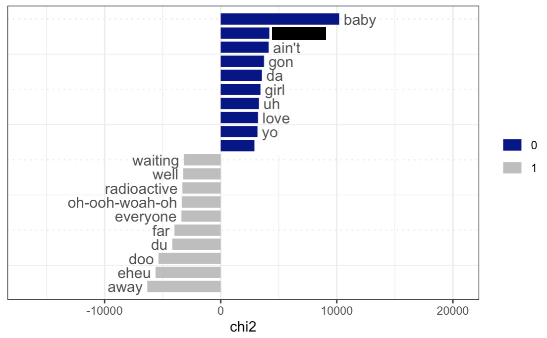
}Keyness plot for the genre “Pop”
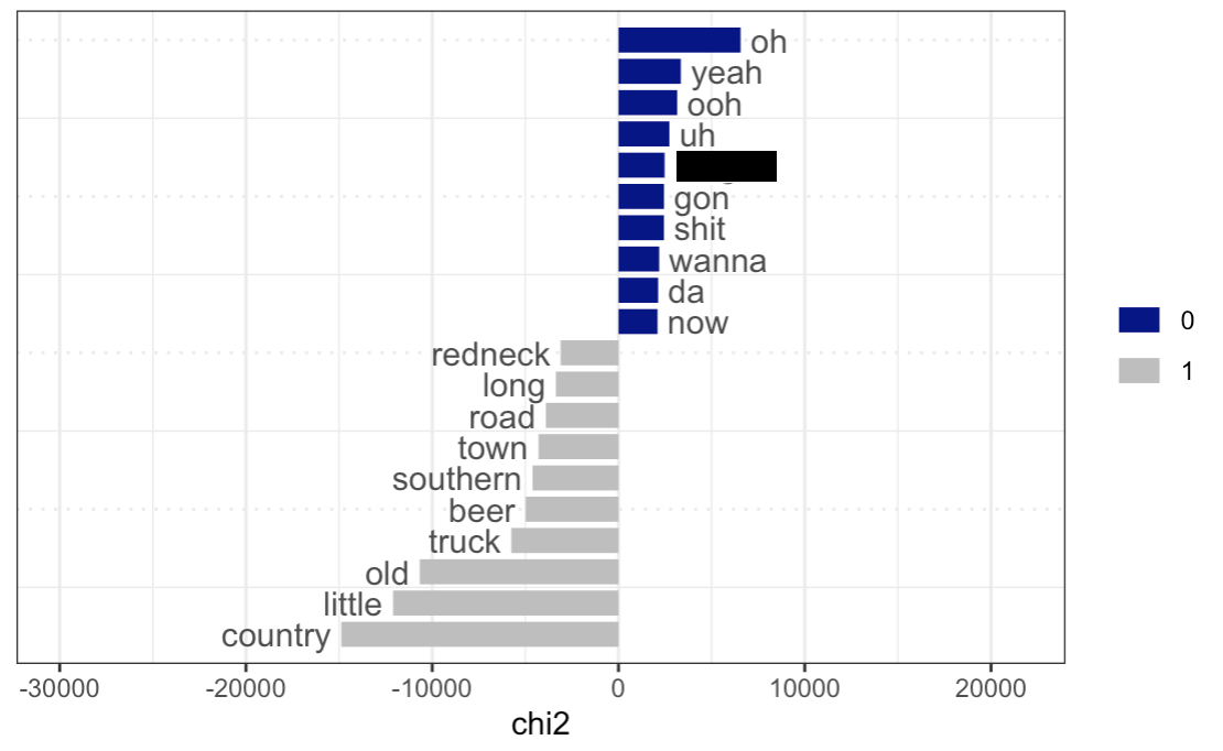
Keyness plot for the genre “Country”
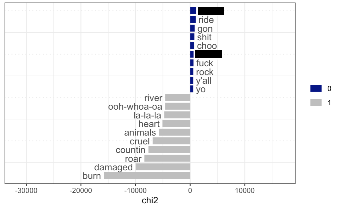
Keyness plot for the genre “Rock”
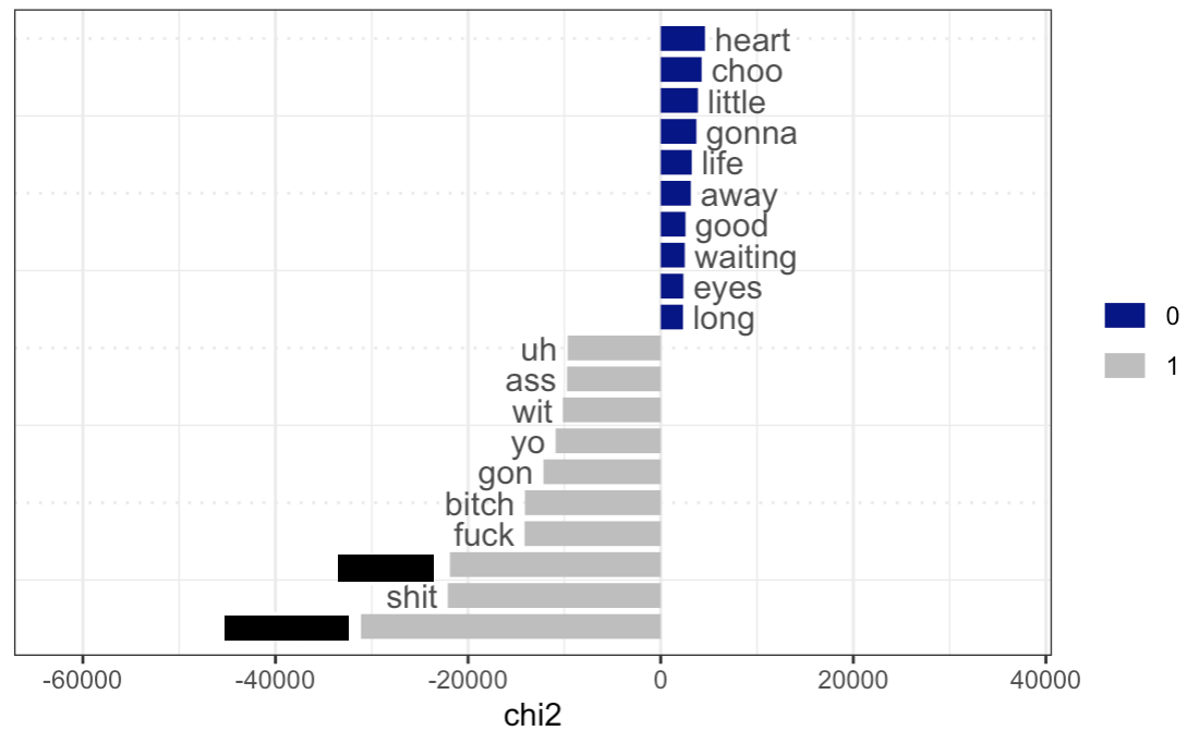
Keyness plot for the genre “Hip-Hop”
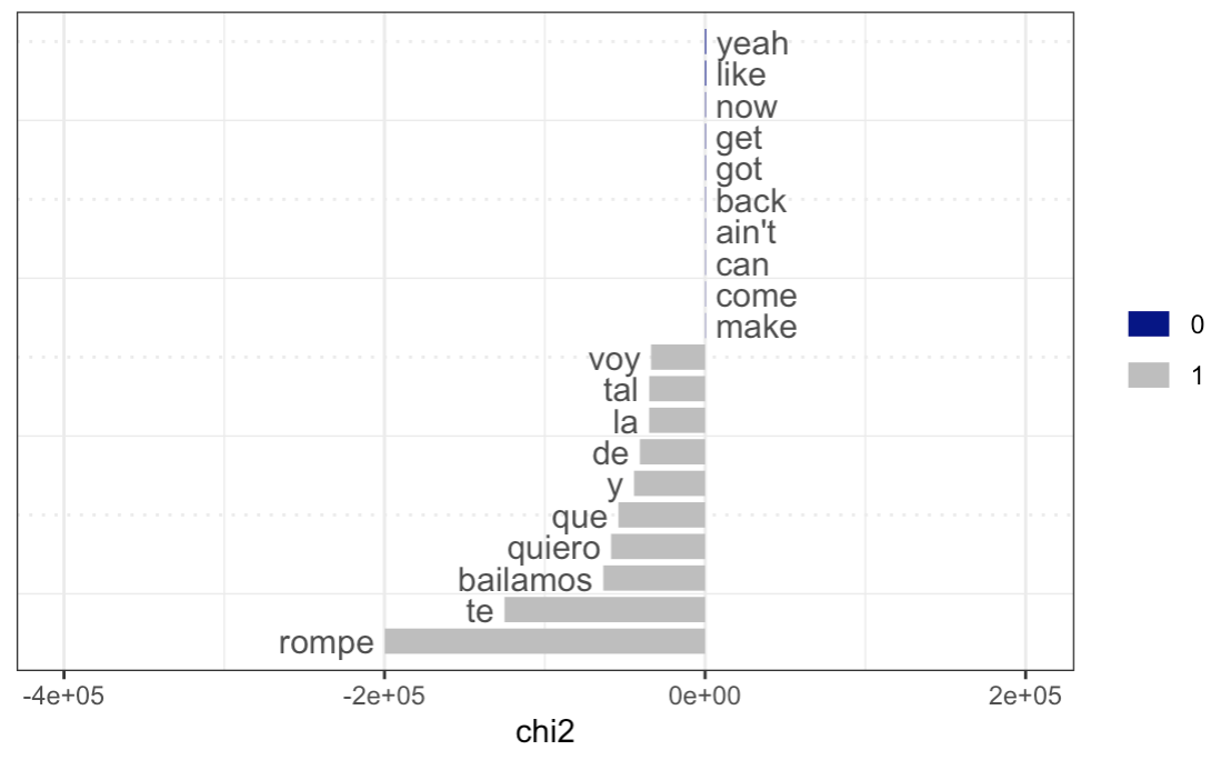
Keyness plot for the genre “Latin”
Keyness plot for the genre “Blues”
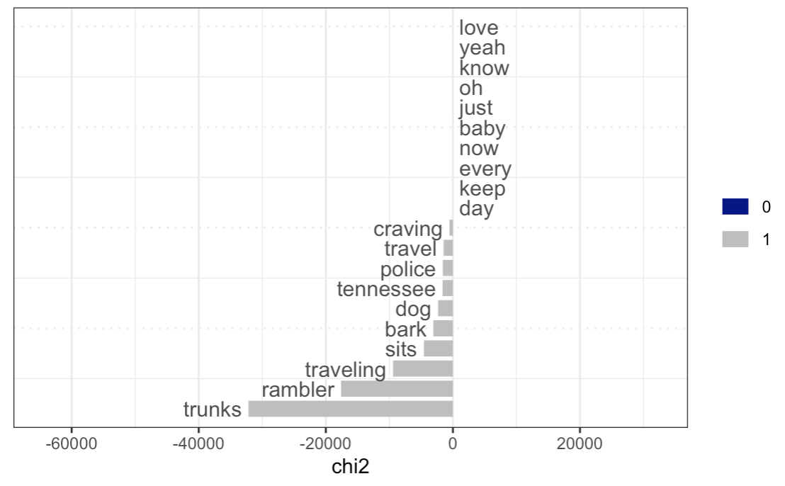
Let us analyze the plots above. Many of the results are quite trivial from common knowledge about certain music genres: for instance, as key words for rap and hip-hop there are racial slurs, curse words, and shortened words (“yo”, “gon”, etc.); for country, we also have a very distinct set of words that reflect the character of this music (“country”, “truck”, “beer”, “southern”, etc.); as for blues, we see “rambler”, “traveling”, “tennessee”, which is again characteristic given the history and the typical content of the genre; in latin, we see a lot of lyrics in Spanish.
In pop music we see “burn”, “damaged”, “roar”, “cruel”, “animals”, “heart” and others. The presence of some of these words makes sense as they are rather common for typical popular songs, however for some of them it is rather difficult to determine the context and tell where they are coming from. This could also be a result of a bias in the dataset.
We see a similar thing for rock music: “away”, “eheu”, “doo”, “everyone”, “oh-ooh-woah-oh”, “radioactive”, etc. It is suggestive that “radioactive” and “oh-ooh-woah-oh” are coming from the song Radioactive by Imagine Dragons that could possibly be overrepresented because it has been popular for a long time, so these words became key words for the genre; some of the others do not make a lot of sense and need to be investigated in context (“eheu”, “doo”, etc.). Some of the others, such as “away”, “everyone” can be genuinely more common for the genre.
Let us look deeper into some of the words mentioned above using the key words in context function to gain a better understanding of why they were selected as key words for certain genres.
kwic(tokens(billboard_corp[docvars(billboard_corp)$genre=="Pop"]), "burn", valuetype = "fixed")[1:10,]
kwic(tokens(billboard_corp[docvars(billboard_corp)$genre=="Pop"]), "damaged", valuetype = "fixed")[1:10,]
kwic(tokens(billboard_corp[docvars(billboard_corp)$genre=="Pop"]), "roar", valuetype = "fixed")[1:10,]
kwic(tokens(billboard_corp[docvars(billboard_corp)$genre=="Pop"]), "cruel", valuetype = "fixed")[1:10,]
kwic(tokens(billboard_corp[docvars(billboard_corp)$genre=="Pop"]), "animals", valuetype = "fixed")[1:10,]
kwic(tokens(billboard_corp[docvars(billboard_corp)$genre=="Pop"]), "heart", valuetype = "fixed")[1:10,]
Let us analyse the plots above. Many of the results are quite trivial from common knowledge about certain music genres: for instance, as key words for rap and hip-hop there are racial slurs, curse words, and shortened words (“yo”, “gon”, etc.); for country, we also have a very distinct set of words that reflect the character of this music (“country”, “truck”, “beer”, “southern”, etc.); as for blues, we see “rambler”, “traveling”, “tennessee”, which is again characteristic given the history and the typical content of the genre; in latin, we see a lot of lyrics in Spanish.
In pop music we see “burn”, “damaged”, “roar”, “cruel”, “animals”, “heart” and others. The presence of some of these words makes sense as they are rather common for typical popular songs, however for some of them it is rather difficult to determine the context and tell where they are coming from. This could also be a result of a bias in the dataset.
We see a similar thing for rock music: “away”, “eheu”, “doo”, “everyone”, “oh-ooh-woah-oh”, “radioactive”, etc. It is suggestive that “radioactive” and “oh-ooh-woah-oh” are coming from the song Radioactive by Imagine Dragons that could possibly be overrepresented because it has been popular for a long time, so these words became key words for the genre; some of the others do not make a lot of sense and need to be investigated in context. Some of the others, such as “away”, “everyone” can be genuinely more common for the genre.
Let us look deeper into some of the words mentioned above using the key words in context function to gain a better understanding of why they were selected as key words for certain genres.
After going through the output of the function for some of the identified key words, the following could be said. It appears that the word “burn” is present as a key word for pop because the songs Afterglow (Ed Sheeran), Counting Starts (One Republic), Burn (Ellie Goulding) that contain the word were present in the chart for an abnormally long time relative to the size of the dataset. A similar thing can be said for the word “damaged” since it is coming from the song “Damaged” (Danity Kane) which was popular for a long time. Unfortunately, most of the other words can also be explained the same way: a song in which the word was used several times was popular for a while, which has led to a bias in the data.
Even though this issue was anticipated from the nature of the dataset (same songs are present more than one time in the dataset if they stay in the chart), I decided not to intervene to preserve the popular music and lyrics that were common at any given period of time. Perhaps, to deal with the issue in further research, one will have to gather data for a wider time period and smaller frequency (use monthly charts instead of weekly ones).
kwic(tokens(billboard_corp[docvars(billboard_corp)$genre=="Rock"]), "away", valuetype = "fixed")[1:200,]
kwic(tokens(billboard_corp[docvars(billboard_corp)$genre=="Rock"]), "everyone", valuetype = "fixed")[1:200,]
kwic(tokens(billboard_corp[docvars(billboard_corp)$genre=="Rock"]), "eheu", valuetype = "fixed")[1:10,]
kwic(tokens(billboard_corp[docvars(billboard_corp)$genre=="Rock"]), "doo", valuetype = "fixed")[1:10,]
kwic(tokens(billboard_corp[docvars(billboard_corp)$genre=="Rock"]), "du", valuetype = "fixed")[1:10,]
kwic(tokens(billboard_corp[docvars(billboard_corp)$genre=="Rock"]), "radioactive", valuetype = "fixed")[1:10,]
Unfortunately, rock music in the dataset has a similar issue, e.g., some words are counted as key words simply because they occurred in songs that stayed in the chart for longer than others. However, I believe that certain words, “everyone” and “away” may be genuinely more characteristic because they were encountered in many different songs across the dataset.
Conclusion
We have found some patterns in music lyrics and their topics depending on time and genre, but the results are rather imperfect for the following reasons. Firstly, it appears that our topic models would mostly identify lyrics that are common within a genre as a standalone topic instead of identifying actual topics in the general meaning of the word, which made it a bit harder to identify topics that are common for each genre. Secondly, there is an issue with songs that stay popular for a long period of time because they have an impact on keyness analysis; however, simply reducing them is tricky because we also need to preserve the popular songs and lyrics at each point in time.
In further research, it would make sense to improve the quality of the dataset taking the drawbacks outlined above into consideration. To elaborate, it would be better to take a larger time frame to introduce more variance and diversity into our data, and reduce the frequency in our data to reduce the repetitions of popular songs, e.g. take the chart published once every 1-2 months instead of charts published every week as in our current dataset. Furthermore, we could experiment further with topic models to improve the quality of identified topics and incorporate this information into research in the context of music sales or social issues. Finally, more techniques could be implemented to study the same data in greater depth, such as sentiment analysis and the analysis of readability and complexity, which were not considered here because of the size limit.