Downloading music artist data using APIs and analyzing audio characteristics in R

Below I present a project that I created as a part of the final assignment for one of my masters courses. In this project, I download data on releases for a given artist that contains titles, dates of releases, audio characteristics of tracks and lyrics using APIs, organize it into a database using SQL, and then create visualizations based on it with ggplot. In this post I will show the code that was used for this project and provide explanations. Access tokens and keys used for APIs are not shown for privacy reasons.

First, load the necessary R packages.

library(httr)
library(tidyverse)
library(geniusr)
library(RSQLite)
library(ggpubr)

We start by downloading releases data using the API of Discogs.com. To do so, first we need to create an app, where we can then find consumer key and consumer secret, which need to be inserted into the code below.

#Type in the name of the artist of interest
artist <- "Nirvana"

#First we are going to retrieve information on releases, e.g., albums and tracks using the API
#of Discogs.com

discogs_key <- 'CONSUMER_KEY'
discogs_secret <- 'CONSUMER_SECRET'

#Obtain the link by inserting the artist name, consumer key and secret
search_url <- sprintf("https://api.discogs.com/database/search?q=%s&key=%s&secret=%s", artist, discogs_key, discogs_secret)

#Make a search query to the API to retrieve the artist ID
search_r <- GET(search_url)

#Parsed content of the page
search_c <- content(search_r, "parsed")

#Retrieve the artist id
id <- search_c$results[[1]]$id

#Obtain the link to retrieve releases by inserting artist ID
releases_url <- sprintf("https://api.discogs.com/artists/%g/releases", id)

#Use the API to obtain releases
releases_r <- GET(releases_url)
 
#Parse the content of the page
releases_c <- content(releases_r, "parsed")

releases <- releases_c$releases

#Create empty lists to turn them into a tibble eventually
release_id_list <- list()
release_title_list <- list()
main_release_list <- list()
year_list <- list()
position_list <- list()
track_title_list <- list()
duration_list <- list()

#Loop through releases and retrieve the values for our columns
for (r in releases){
  relid <- r$id
  reltitle <- r$title
  main_release <- r$main_release
  year <- r$year
  
  #Get the link for the release 
  rel_url <- r$resource_url

  #Access it through API
  rel_r <- GET(rel_url)

  #Parse the content of the link
  rel_c <- content(rel_r, "parsed")

  tracklist <- rel_c$tracklist
  
  #Loop through the tracks in the release
  for (t in tracklist){
    position <- t$position
    title <- t$title
    duration <- t$duration
    
    release_id_list <- append(release_id_list, relid)
    release_title_list <- append(release_title_list, reltitle)
    main_release_list <- append(main_release_list, main_release)
    year_list <- append(year_list, year)
    position_list <- append(position_list, position)
    track_title_list <- append(track_title_list, title)
    duration_list <- append(duration_list, duration)
  }
}

#Create a tibble containing all the tracks by the artist
discogs_features <- tibble(
  release_id = unlist(release_id_list),
  release = unlist(release_title_list),
  year = unlist(year_list),
  position = unlist(position_list),
  title = unlist(track_title_list),
  duration = unlist(duration_list)
)
 
discogs_features$artist <- artist

#Create a column with unique IDs for each track by combining release ID and position so we can
#use this later to join tables
discogs_features <- discogs_features %>%
  mutate(unique_id = paste(release_id, position, sep = "_"))

Next, we are going to access the API of Spotify to retrieve audio characteristics of the tracks we just downloaded.

#Create an empty tibble we are going to bind rows to
spotify_features <- tibble(
  danceability = numeric(), 
  energy = numeric(), 
  key = numeric(), 
  loudness = numeric(), 
  mode = numeric(), 
  speechiness = numeric(), 
  acousticness = numeric(),
  instrumentalness = numeric(), 
  liveness = numeric(), 
  valence = numeric(), 
  tempo = numeric(), 
  type = character(), 
  id = character(), 
  uri = character(), 
  track_href = character(), 
  analysis_url = character(), 
  duration_ms = numeric(), 
  time_signature = numeric())

#Getting the access token for Spotify API
response <- POST(
  "https://accounts.spotify.com/api/token",
  config = authenticate(user = "CLIENT_ID", 
                        password = "SECRET"),
  body = list(grant_type = "client_credentials"), 
  encode = "form"
)

token <-  content(response) 
bearer_token <- paste(token$token_type, token$access_token)

After that we loop through the table obtained using the Discogs.com API and get the corresponding audio information from the Spotify API. We also add a column with Spotify song IDs to the original Discogs table to that we will be able to join these tables later.

for (i in 1:nrow(discogs_features)){
  #Get the title of the track and the name of the artist
  title <- discogs_features$title[i]
  artist <- discogs_features$artist[i]
  
  #Get the unique ID so that we can later join the Spotify table with the Discogs table
  unique_id <- discogs_features$unique_id[i]
  
  #We need to modify the names of the artist and the track to insert them into the search
  #query properly
  title_mod <- str_c(str_split(title, " ")[[1]], collapse = "%20")
  artist_mod <- str_c(str_split(artist, " ")[[1]], collapse = "%20")
  
  #Get the search URL
  search_url <- paste("https://api.spotify.com/v1/search?q=track:", title_mod, "%20artist:", artist_mod, "&type=track")
  
  search_url <- str_replace_all(search_url, " ", "")
  try({
    #Make a search through API to obtain the ID of the track
    search_r <- GET(search_url, config = add_headers(Authorization = bearer_token))
    
    #Parse the content of the page
    search_c <- content(search_r, "parsed")
    
    #If the search didn't find anything, skip
    if (length(search_c$tracks$items) == 0){
      next
    } else {
      #Get the track ID
      trid <- search_c$tracks$items[[1]]$id
      
      if (is.null(trid) == FALSE){
        #Insert the ID into our link for retrieving audio features
        tr_url <- sprintf("https://api.spotify.com/v1/audio-features/%s", trid)
        

        #Get the audio features
        tr_r <- GET(tr_url,config = add_headers(Authorization = bearer_token))
          
        #Transform them into a tibble
        tr_features <- as_tibble(content(tr_r))
        
        #Add the ID from Discogs table
        tr_features$discogs_id <- unique_id
        
        #Bind the newly obtained tibble to the one initially created
        spotify_features <- bind_rows(spotify_features, tr_features)
          
        spotify_id_list <- append(spotify_id_list, trid)

      } else {
        next
      }
    }
  }, silent = TRUE)
}

spotify_features <- spotify_features %>%
  filter((is.na(danceability) == FALSE) & (is.na(discogs_id) == FALSE))

Now we are going to download the lyrics of the tracks we downloaded above. To do so, we will use the API of Genius.

Sys.setenv(GENIUS_API_TOKEN = "TOKEN")

#Search for information on the artist
genius_artist_tib <- search_artist(artist)

#Retrieve their ID
genius_artist_id <- genius_artist_tib$artist_id

#Get a dataframe containing all of their songs and information on them
genius_songs <- get_artist_songs_df(genius_artist_id) 

#Initialize an empty column to store lyrics for each song
genius_songs_lyrics <- tibble()
genius_songs$lyrics <- NA

get_lyrics <- function(id){
  lyrics_tib <- get_lyrics_id(id)
  lyrics <- str_c(lyrics_tib$line, collapse = " ")
  return(lyrics)
}

#Loop through the songs dataframe and get lyrics
for (i in 1:nrow(genius_songs)){
  try({
    genius_songs[i,8] <- get_lyrics(genius_songs$song_id[i])
  }, silent = TRUE)
}
 
genius_songs <- genius_songs %>%
  filter(is.na(lyrics) == FALSE)

Finally, we have three tables containing data we downloaded using APIs (Note: I did not download data on releases using the Spotify API directly for convenience because some technical issues were encountered). Next, we are going to create a database using RSQLite and add our tables to it.

#Creating the database
db <- dbConnect(RSQLite::SQLite(), "lyrics_audio_characteristics.sqlite")

#Writing tables
dbWriteTable(db, "discogs", discogs_features, overwrite = TRUE)
dbWriteTable(db, "spotify", spotify_features, overwrite = TRUE)
dbWriteTable(db, "genius", genius_songs, overwrite = TRUE)

To make the most out of the data in our database and to create more meaningful visualizations, we will need to join our tables by using mutual columns. The creation of such columns was highlighted in the code chunks above. In the chunk below I will show what joins can be performed on our data.

#We can join the Discogs and Spotify tables by using the unique ID column that we created above
dbGetQuery(db, "SELECT *
           FROM discogs
           JOIN spotify
           ON discogs.unique_id = spotify.discogs_id
           LIMIT 5")

#We can join the Discogs and Genius tables by using the song names
dbGetQuery(db, "SELECT *
           FROM discogs
           LEFT JOIN genius
           ON discogs.title = genius.song_name
           LIMIT 5")

#We can also join all tables
dbGetQuery(db, "SELECT * FROM
           (SELECT *
           FROM discogs
           LEFT JOIN genius
           ON discogs.title = genius.song_name) j
           JOIN spotify s
           ON j.unique_id = s.discogs_id
           LIMIT 5")

In the next section we are going to join the tables in our database and load the joined table from SQLite into R in order to work with it. We will use it later to create visualizations and analyze the data.

joined_table <- dbGetQuery(db, "SELECT * FROM
           (SELECT *
           FROM discogs
           LEFT JOIN genius
           ON discogs.title = genius.song_name) j
           JOIN spotify s
           ON j.unique_id = s.discogs_id")

#Disconnect from the database
dbDisconnect(db)

#Filter out the rows that have no lyrics
joined_table <- joined_table %>%
  filter(is.na(lyrics) == FALSE) 

joined_table$duration_ms <- as.numeric(joined_table$duration_ms)

#Set levels so that albums don't get sorted alphabetically
joined_table$release <- factor(joined_table$release, levels = unique(joined_table$release))

#Group the data by album
grouped_album <- joined_table %>%
  group_by(release)

#Calculate average audio characteristics for each album
albums_summ <- grouped_album %>% summarise(
  mean_danc = mean(danceability),
  mean_energy = mean(energy),
  mean_loud = mean(loudness),
  mean_valence = mean(valence),
  mean_temp = mean(tempo),
  mean_duration = mean(duration_ms)
)

In the following block of code I create bar plots for some of the audio characteristics from the Spotify API. The charts display average audio characteristics by album; albums are arranged in order of release.

danceability_plot <- ggplot(albums_summ, aes(fill = release, y = mean_danc, x = release)) +
  geom_bar(position="dodge", stat="identity") +
  labs(y = "",
       x = "Danceability",
       fill = "Releases") +
  theme(axis.text.x=element_blank(),
        axis.ticks.x=element_blank(),
        axis.ticks.y=element_blank(),
        legend.position = "none")

energy_plot <- ggplot(albums_summ, aes(fill = release, y = mean_energy, x = release)) +
  geom_bar(position="dodge", stat="identity") +
  labs(y = "",
       x = "Energy",
       fill = "Releases") +
  theme(axis.text.x=element_blank(),
        axis.ticks.x=element_blank(),
        axis.ticks.y=element_blank(),
        legend.position = "none") 

loudness_plot <- ggplot(albums_summ, aes(fill = release, y = mean_loud, x = release)) +
  geom_bar(position="dodge", stat="identity") +
  labs(y = "",
       x = "Loudness",
       fill = "Releases") +
  theme(axis.text.x=element_blank(),
        axis.ticks.x=element_blank(),
        axis.ticks.y=element_blank(),
        legend.position = "none") 
 
valence_plot <- ggplot(albums_summ, aes(fill = release, y = mean_valence, x = release)) +
  geom_bar(position="dodge", stat="identity") +
  labs(y = "",
       x = "Valence",
       fill = "Releases") +
  theme(axis.text.x=element_blank(),
        axis.ticks.x=element_blank(),
        axis.ticks.y=element_blank(),
        legend.position = "none") 

tempo_plot <- ggplot(albums_summ, aes(fill = release, y = mean_temp, x = release)) +
  geom_bar(position="dodge", stat="identity") +
  labs(y = "",
       x = "Tempo",
       fill = "Releases") +
  theme(axis.text.x=element_blank(),
        axis.ticks.x=element_blank(),
        axis.ticks.y=element_blank(),
        legend.position = "none") 

duration_plot <- ggplot(albums_summ, aes(fill = release, y = mean_duration, x = release)) +
  geom_bar(position="dodge", stat="identity") +
  labs(y = "",
       x = "Duration",
       fill = "Releases") +
  theme(axis.text.x=element_blank(),
        axis.ticks.x=element_blank(),
        axis.ticks.y=element_blank(),
        legend.position = "none") 

plot <- ggarrange(danceability_plot, energy_plot, loudness_plot, 
                  valence_plot, tempo_plot, duration_plot, ncol = 3, nrow = 2, 
                  common.legend = TRUE, legend = "right")

annotate_figure(plot, top = text_grob("Mean values of Spotify audio characteristics by release"))

The illustration below is the output of the last code chunk.

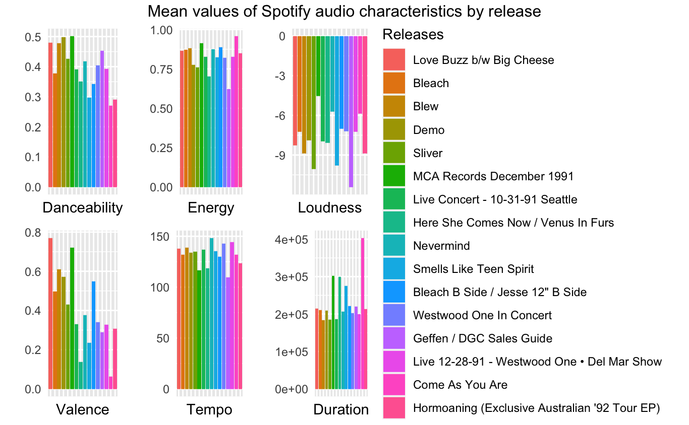
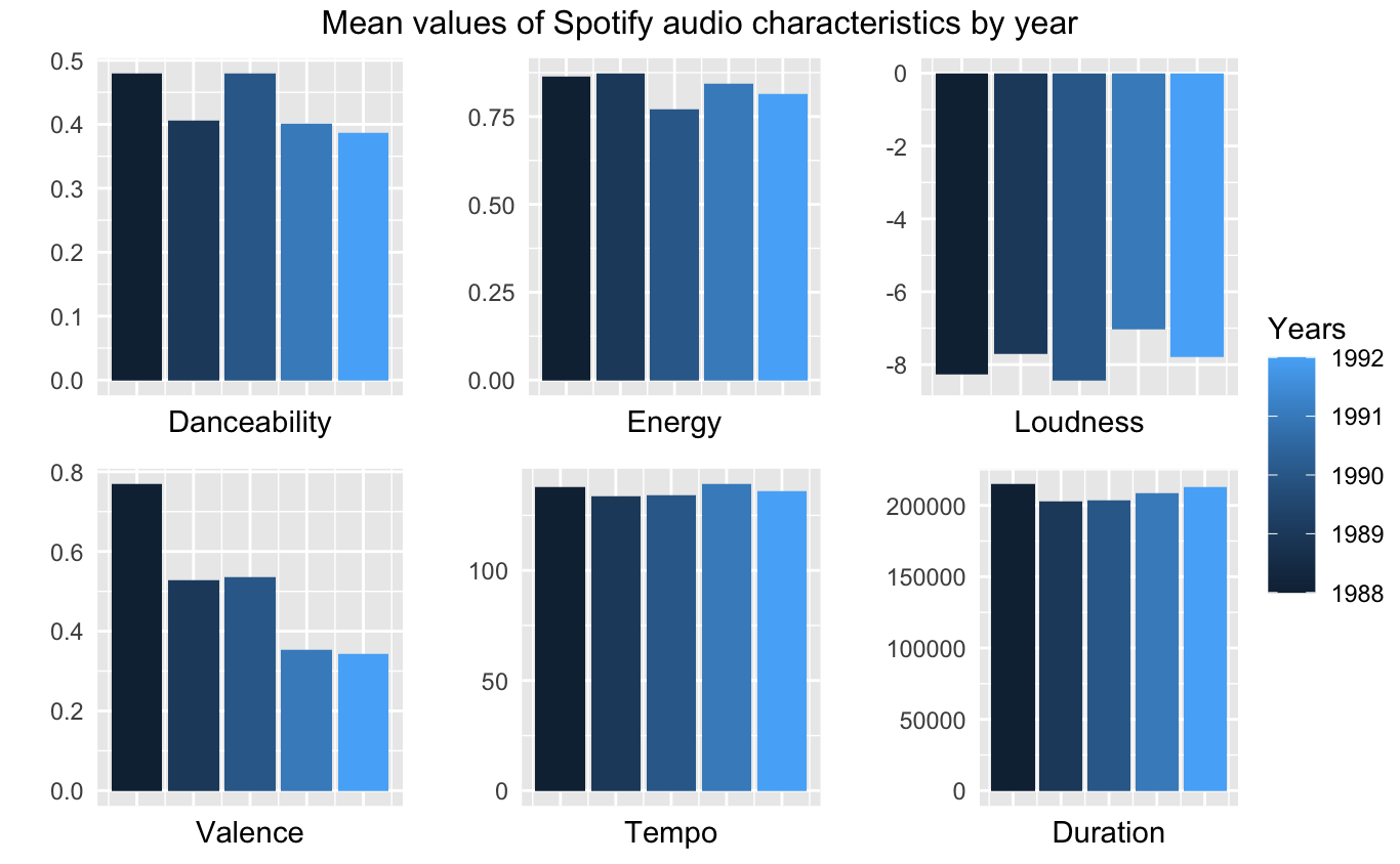
Next I am going to show a similar visualization, but this time the average audio characteristics are calculated by year. First, we regroup the joined table and modify the data.

#Group the data by year
grouped_year <- joined_table %>%
  group_by(year)

#Calculate average audio characteristics for each year
years_summ <- grouped_year %>% summarise(
  mean_danc = mean(danceability),
  mean_energy = mean(energy),
  mean_loud = mean(loudness),
  mean_valence = mean(valence),
  mean_temp = mean(tempo),
  mean_duration = mean(duration_ms)
)

Next, we create the plots.

danceability_plot <- ggplot(years_summ, aes(fill = year, y = mean_danc, x = year)) +
  geom_bar(position="dodge", stat="identity") +
  labs(y = "",
       x = "Danceability",
       fill = "Years") +
  theme(axis.text.x=element_blank(),
        axis.ticks.x=element_blank(),
        axis.ticks.y=element_blank(),
        legend.position = "none")

energy_plot <- ggplot(years_summ, aes(fill = year, y = mean_energy, x = year)) +
  geom_bar(position="dodge", stat="identity") +
  labs(y = "",
       x = "Energy",
       fill = "Years") +
  theme(axis.text.x=element_blank(),
        axis.ticks.x=element_blank(),
        axis.ticks.y=element_blank(),
        legend.position = "none") 

loudness_plot <- ggplot(years_summ, aes(fill = year, y = mean_loud, x = year)) +
  geom_bar(position="dodge", stat="identity") +
  labs(y = "",
       x = "Loudness",
       fill = "Years") +
  theme(axis.text.x=element_blank(),
        axis.ticks.x=element_blank(),
        axis.ticks.y=element_blank(),
        legend.position = "none") 

valence_plot <- ggplot(years_summ, aes(fill = year, y = mean_valence, x = year)) +
  geom_bar(position="dodge", stat="identity") +
  labs(y = "",
       x = "Valence",
       fill = "Years") +
  theme(axis.text.x=element_blank(),
        axis.ticks.x=element_blank(),
        axis.ticks.y=element_blank(),
       legend.position = "none") 

tempo_plot <- ggplot(years_summ, aes(fill = year, y = mean_temp, x = year)) +
  geom_bar(position="dodge", stat="identity") +
  labs(y = "",
       x = "Tempo",
       fill = "Years") +
  theme(axis.text.x=element_blank(),
        axis.ticks.x=element_blank(),
        axis.ticks.y=element_blank(),
        legend.position = "none") 

duration_plot <- ggplot(years_summ, aes(fill = year, y = mean_duration, x = year)) +
  geom_bar(position="dodge", stat="identity") +
  labs(y = "",
       x = "Duration",
       fill = "Years") +
  theme(axis.text.x=element_blank(),
        axis.ticks.x=element_blank(),
        axis.ticks.y=element_blank(),
        legend.position = "none") 

plot <- ggarrange(danceability_plot, energy_plot, loudness_plot, 
                  valence_plot, tempo_plot, duration_plot, ncol = 3, nrow = 2, 
                  common.legend = TRUE, legend = "right")

annotate_figure(plot, top = text_grob("Mean values of Spotify audio characteristics by year"))

Below you can see the corresponding illustration.

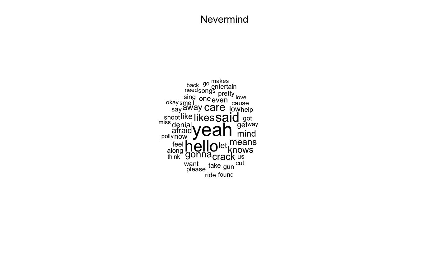
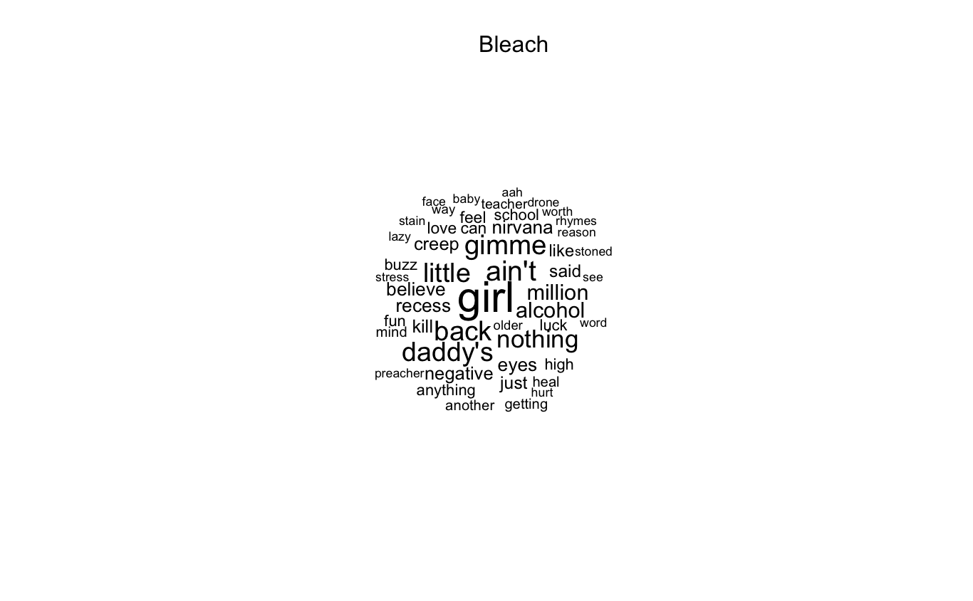
Next I am going to switch to a different type of visualization: wordclouds. We will use the data gathered using the Genius API for that.

lyrics_documents <- c()

for (r in unique(joined_table$release)){
  #Get the rows for the given release
  dt_release <- joined_table[joined_table$release == r, ]
  
  #Concatenate the lyrics into a document
  doc <- str_c(dt_release$lyrics, collapse = " ")
  
  #Add to the list of documents
  lyrics_documents <- append(lyrics_documents, doc)
}
 
names(lyrics_documents) <- unique(joined_table$release)

#Create a corpus
lyrics_corpus <- corpus(lyrics_documents, 
                        docvars = data.frame(name = names(lyrics_documents),
                                             characters = str_count(lyrics_documents)))

#Clean the corpus
lyrics_corpus_cleaned <- lyrics_documents %>%
  tokens(remove_punct = TRUE) %>%
  tokens_remove(stopwords('en')) %>%
  dfm() %>%
  dfm_subset(ntoken(lyrics_corpus)>0)
 
#Create a wordcloud for each release
for (i in 1:nrow(lyrics_corpus_cleaned)){
  print(textplot_wordcloud(lyrics_corpus_cleaned[i,], color = 'black',
                            rotation = 0, min_size = .75, max_size = 3, max_words = 50))
  print(mtext(docnames(lyrics_corpus_cleaned[i,])))
}

#Disconnect from the database
dbDisconnect(db)

The code above creates a wordcloud for each release, but since some of the releases in this case are live albums and demos, some patters are repeating. For this reason, I am going to show wordclouds for only some of the albums, which will be shown below.